Advanced Edge Detection Techniques Using Python

**Edge Detection and Its Roots in Neuroscience** Artificial intelligence has taken significant leaps in recent years, permeating many aspects of both our professional and personal lives. Today, virtually every major large language model is influenced by that seminal transformer paper—a brief but revolutionary work that has stirred excitement and trepidation throughout the tech community. It’s hard to overstate how this framework has transformed AI in such a short time. What’s fascinating is how deeply this shift has also affected the realm of computer vision. Vision-language models (VLMs) have surged in popularity, proving capable of generalizing across an impressive spectrum of tasks—from segmentation to image generation. These models have not only outperformed their predecessors in benchmark tests but have done so with minimal tuning, altering the expectations of what AI can achieve. But let’s not get ahead of ourselves. This enthusiastic embrace of transformer architectures shouldn't obscure the fact that they might not be the only—or even the best—path toward advancing AI as we know it. After all, we’re still grappling with fundamental issues, like AI’s struggles with basic tasks such as accurately counting letters in simple words. Alternatives like neuromorphic computing and photonic neural networks are emerging, each providing unique avenues toward refining how we create intelligent systems. Today, I’m pivoting our focus to a foundational concept that has shaped both our understanding of visual perception and the algorithms we employ to replicate it in machines: edge detection. My thoughts on this were profoundly influenced by David Marr's influential book, *Vision*. Marr intertwined various domains—neurophysiology and computer vision—contributing to an analytical approach that remains relevant today. In this article, we’ll dive into different algorithms employed for edge detection in images and highlight their intriguing parallels with how our nervous systems process visual information. **Understanding Marr’s Contributions** David Marr’s work offers a lens through which we can appreciate how computers interpret visual scenes. He proposed a three-level framework that describes information-processing systems effectively: 1. **Computational Level**: This addresses what problem is being solved and the reasoning behind it. For instance, edge detection falls under this category. 2. **Algorithmic Level**: This pertains to the specific methods used to solve the problems identified at the computational level—like the Laplacian transform for edges. 3. **Implementational Level**: This discusses where and how these computations occur, whether in biological systems or artificial ones. Marr’s insistence that these levels are interdependent made his framework not just useful, but essential for understanding complex systems. He argued that a holistic examination is necessary to truly grasp how visual processing occurs, which has made his ideas resonate across scientific communities for decades. The text contains captivating insights into topics like random dot stereograms and motion perception—definitely a must-read for anyone curious about the intersection of science and technology. Next, we’ll unravel the key concepts related to edge detection that stem from this structured approach, providing clarity on how these principles can be applied practically. **The Essence of Zero-Crossing in Edge Detection** From a computational viewpoint, edges signify spatial discontinuities within images. If you visualize a simple grayscale image, you’ll spot edges wherever transitions from light to dark and vice versa occur. These abrupt changes in pixel intensity inspire a logical strategy—calculating image gradients akin to derivatives. The first derivative reveals stark transitions, producing recognizable peaks (in a shift from dark to light) or troughs (for light to dark). However, it’s the second derivative that brings clarity to this process, pinpointing zero-crossings exactly at these edges. This principle is what underpins zero-crossing methods in edge detection. Marr and his colleague Hildreth proposed the Laplacian of Gaussian (LoG) as a pivotal operator in this context. The Laplacian is a mathematical construct that combines second-order derivatives across spatial dimensions, helping to pinpoint where rapid changes occur. When the Laplacian is employed directly on noisy images, it amplifies minor fluctuations in intensity. To counteract this noise, a Gaussian pre-filter comes into play, smoothing the image before any differentiation happens. Through convolution properties, these steps can be merged into one operation—the LoG, characterized by its unique shape that captures those vital zero-crossings at edges. In Marr's exploration of visual perception, he linked the organization of retinal ganglion cells—akin to the Difference of Gaussians (DoG) model—to the mathematical representation of the LoG. This means our retinas are subconsciously processing edge information long before it reaches our brains for higher-level interpretation. The alignment between computational theories and biological data stands as one of the most convincing examples bridging neuroscience and advanced algorithms. While zero-crossing methods are elegantly theoretical, the reality of edge detection largely relies on gradient methods—the workhorses of computer vision. So, let’s delve deeper into how these image gradients are computed and their practical applications in modern algorithms.

Understanding Gradient Operators

The Prewitt operator is a foundational edge detection technique that emphasizes uniformity in neighbor weighting. It functions through two matrices representing gradients in the x and y directions. This can be encapsulated as follows: The matrices here illustrate that the Prewitt operator treats all neighboring pixels equally. When applied, these operators yield a gradient magnitude at every pixel: The resulting gradient direction can be determined by the equation: . Higher gradient magnitudes indicate significant changes in intensity, suggesting that an edge may be present, whereas smaller values denote uniform areas. However, one major limitation of both Prewitt and Sobel operators is their susceptibility to noise. They tend to produce edges that are not sharp, often leading to misleading results as they flag all pixels with high gradient values, regardless of whether they correspond to true edges. This characteristic is precisely the issue that John Canny aimed to rectify with his edge detection algorithm.

Canny Edge Detection: A Decisive Breakthrough

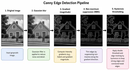
John Canny’s pioneering work in 1986, detailed in his paper *A Computational Approach to Edge Detection*, revolutionized the field with its structured approach to edge detection. Where earlier operators were reactive to noise and imprecise with edge localization, Canny introduced a method that optimized detection through three criteria: minimizing missed edges, reducing false positives, and ensuring unique edge responses. The algorithm is executed in a systematic, four-step process:

Step 1 – Gaussian Smoothing

Noise reduction is the priority in the initial step, achieved through the application of a Gaussian filter. The width of this filter, represented by , controls the balance between detail preservation and noise suppression. A larger results in better noise handling but can blur critical features.

Step 2 – Gradient Computation

Following the smoothing operation, the gradient of the image is computed, usually employing Sobel kernels. This two-part process evaluates both the magnitude and the direction at pixel levels.

Step 3 – Non-Maximum Suppression (NMS)

To refine edge definition, Canny’s algorithm applies Non-Maximum Suppression. This phase thins detected edges by evaluating whether each pixel is a local maximum in the direction of the gradient, pruning those that do not meet this criterion.

Step 4 – Hysteresis Thresholding

The concluding step leverages dual thresholds—high and low—to finalize edge detection. Pixels exceeding the high threshold are confirmed as edges, while those below the low threshold are discarded. Pixels that fall between the two thresholds may be classified as edges if they connect to strong ones, ensuring the coherence and continuity of detected edges amidst gradient inconsistencies. As visualized in the following image, the Canny process systematically addresses the pitfalls identified in prior methods, enhancing performance in noise-heavy environments while maintaining edge integrity. A thorough grasp of the Canny edge detection pipeline is essential for implementing robust image processing techniques that withstand the challenges posed by real-world data input.

Final Thoughts on Edge Detection

When you strip down the complexities of image processing, at its heart lies the fundamental principle of edge detection. We've navigated through the evolution of techniques, tracing an intellectual lineage from the biological inspiration of retinal ganglion cells to the mathematical elegance of the Canny edge detector. This journey isn’t merely academic; it’s deeply practical and reflects how foundational concepts can inform modern applications. Here's the thing: despite advances in deep learning and the allure of end-to-end vision systems, the core tenets of edge detection remain indispensable. The methods we've discussed demonstrate that even in a landscape dominated by neural networks, there’s still a critical role for classical techniques. Take, for example, the Gaussian scale-space theory. Its emphasis on scale is not just theoretical; it’s practical. The options between coarse and fine scales translate to tangible outcomes in visual clarity and detail retention. Which brings us to another key insight: the balance between noise reduction and edge recovery. As we've illustrated, lower thresholds in hysteresis can amplify noise, while higher thresholds might yield sleek visuals at the cost of losing intricate details. This duality raises strategic questions for engineers and researchers alike: how do you tailor these parameters to best suit your specific application, whether it’s in autonomous driving systems, medical imaging, or industrial inspections? Looking forward, it’s clear that while computational methods continue to advance, the foundational approach of edge detection will persist. Its principles will integrate with newer technologies, potentially hybridizing traditional methods with emerging neural solutions. It’s this synergy between classic and modern that will undoubtedly lead to new breakthroughs in image processing. So, if you’re in this space, be prepared to lean on these age-old techniques while innovating with the latest advancements. They might just be the linchpin for your next project or breakthrough. Thanks for following along on this exploration—stay curious and keep pushing the boundaries of what’s possible!